Recursion is a concept that often used in programming. Usually, when people said the problem could be solved recursively - they meant the problem could be broken down into a smaller problem.
A lot of the algorithms and data structures are usually solved in iteratively and recursively.
A lifecycle of project management usually are conducting in an iterative approach. An extensive system can be broken down into multiple microservices. The most popular data structure, arrays, is a recursive data structure by nature.
For instance, imagine you are having a coding interview for an X company, and they ask you about the classic Fibonacci questions.
“Given a number n, print nth Fibonacci Number.”
The first thing that pops in your head about solving this problem is either recursively or iteratively (Dynamic Programming). However, there is also another way of answering these questions using corecursion.
You must be thinking:
“So, what is Corecurion?”
In this article, I will share what corecursion is and give you two examples of solving problems with corecursion.
What is Corecursion?
Said, corecursion is the opposite of recursion. Whereas, recursion consumes data, corecursion produces data.
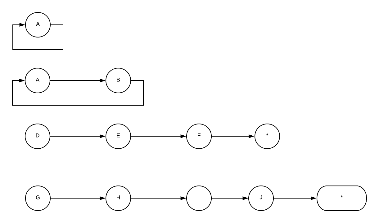
Recursion usually works analytically. Starting from the data or problem that is further from the base case, you break down the problem into a smaller data by using induction until it hits the base case.
Corecursion works synthetically. Starting from the base case and build it up - iteratively produces data further away from the base case with some recurrence relation.
A classic function of corecursion is unfold:
def unfold[A,S](s: S)(f: S => Option[(A,S)]): List[A]
The A is the result of the state after applying f, and S is the current state or next state after using f.
It takes an initial state, and a function for producing both the next state and the future value in the generated iterator, be it List or Stream.
One way of thinking about recursion vs. corecursion is to solve the problem as a top-down approach and a bottom-up approach.
Let’s implement unfold:
def unfold[A,S](s:S)(f: S => Option[(A,S)]): List[A] = f(s) match {
case Some((currentResult,nextState)) => currentResult :: unfold(nextState)(f)
  case None => Nil
}
With the classic Fibonacci number, we can generate n Fibonacci number with unfolding by starting from 0 and 1 and adding both numbers to produce the next state:
def fib(n:Int): Int = generateFibSequence(n).last


def generateFibSequence(n:Int): List[Int] =
  unfold((n, (0,1))){s => s match {
    case ((num, (f0, f1))) if(num > 0) => Some((f0, (num -1, (f1, f0+f1))))
    case _ => None // terminate
  }}
In the above function, we generate a Fibonacci sequence by keeping track of the n number and two of the previous state to produce the next Fibonacci state. The function will terminate when num reaches 0, meaning we provide n Fibonacci sequence.
Corecursive are often widely used in functional programming, primarily when dealing with an infinite data structure, such as Stream-building function. Often, corecursion gives the solution of producing a finite subset of a potentially infinite structure, such as creating Generator.
I will give two other examples where we can use corecursion to solve the problem.
Factorial
A recursion computing is of factorial will define a base case of factorial(0) equals 1, and the recurrence relation will be n * factorial(n-1)*.
With corecursion, we start with the base case, factorial(0) which is 1. To get to the next result, n = 1.
Just like regular iterative solution, factorial(2) can be derived from factorial(1) * (1+1). factorial(1) can be derived from factorial(0) * (0+1), which is the base case.
Therefore, we can read backward by saying - “factorial(n+1) can be produced by having factorial(n) multiple by n+1”.
By knowing the next value and the next state, let’s write the solution for this problem with unfold:
def factorialGenerator(n:Int): List[Int] = unfold((1, 1)){
  case ((num,_)) if (num > n) =>  None
  case ((num, currFactorial)) =>
    val nextFactorialValue = currFactorial * num
    Some(( nextFactorialValue, (num+1, nextFactorialValue)))

}
The unfold function will take in a tuple of the n value and the current factorial. Therefore, we increase the n value while computing our next factorial number. The call back functions within unfold with taking the future value and the next state. The next value will be currentFactorial x num, and the next state will be a tuple of the following number and the next evaluated factorial.
Tree Traversal
Tree traversal in the depth-first search approach is a classic example of recursion. However, tree traversal in a breadth-first search approach can be implemented using corecursion.
The ultimate difference in implementing depth-first and breadth-first lies in the data structure that you store the nodes. We are storing each node with a stack (LIFO) as we traverse down the tree with a depth-first search. With breadth-first search, we store the nodes with a queue (FIFO) as we traverse down the tree.
It is recursively using a depth-first search in post-order traversal fashion. It starts from the root and recursively traversing each child’s subtree in turn.
Using corecursion to implement the breadth-first search, you can start from the root, and generate all its subtree and put all its subtree as a whole list on the next state. The following state act as a queue to traverse to.
Let’s implement BFS with unfold in a node:
sealed trait Graph[+T]
case class Node[T](value:T, child:List[Graph[T]]) extends Graph[T]


  def bfs[T](root:Graph[T]): List[T] =
    unfold(List(root)){
      case Node(value,child) :: t =>
        val newQueue = t ++ child
        Some((value, newQueue))
      case Nil => None
    }
On each step of the unfold function, we will return the head as the new result, and the newQueue as the next state. We will append the child of the root on the existing list of “queue”.
Recursive traversal handles the leaf node as the base case and analyzes a tree into a subtree. By contrast, corecursion traversal handles the root node as the base case and treats the tree as a synthesized root node and its children. It produces an auxiliary output a list of subtree at each step, giving input to the next level. The child node of the root will become the root node on the next step.
Takeaway
If we are dealing with an infinite structure of trees or generating unlimited structure of Fibonacci, or factorial, corecursion shows usefulness rather the recursion. Through recursion, it will never reach the base case since it is infinite. Whereas, corecursion will start from the base case and produces its output infinitely.
The generic function of corecursion is the essence of unfold. To unfold is to enumerate elements so that the given item is the same relation to its precedent and the precedent to one part before.
Another way of deriving corecursion is by using iteration, or bottom-up approach. In functional programming, corecursion has been slowly defined through stream-building function.
All source for the code are here.